Count Sketch
Shusen Wang, wssatzju@gmail.com
Count sketch stems from the streaming literature in the theoretical computer science society, and it has been a popular matrix sketching method since the following paper.
Kenneth L. Clarkson and David P. Woodruff. Low rank approximation and regression in input sparsity time. In STOC, 2013.
The beauty of the count sketch is that given ${\bf A}\in \mathbb{R}^{m\times n}$, a sketch of any size can be formed in $O( \textrm{nnz} ({\bf A}) )$ time, where $\textrm{nnz} ({\bf A})$ denotes the number of non-zero entries in ${\bf A}$.
In this article we provide intuitive descriptions of the count sketch and three ways of implentation.
1. Preparations
We first prepare the data for our experiments. Let us load a matrix from the file '../data/letters.txt', which has $15,000$ samples and $16$ features.
# prepare data
import numpy as np

# load matrix A from file
filepath = '../data/letters.txt'
matrixA = np.loadtxt(filepath).T
print('The matrix A has ', matrixA.shape[0], ' rows and ', matrixA.shape[1], ' columns.')
2. Algorithm Description
Suppose we are given any fixed matrix ${\bf A} \in \mathbb{R}^{m\times n}$ and the size of sketch $s$. We first hash each column with a discrete value which is uniformly sampled from $\{1, \cdots , s\}$, then flip the sign of each column with probability 50%, and finally sum up the columns with the same hash value. The result is an $m\times s$ matrix ${\bf C} = {\bf AS}$.
The image below illustrates the procedure of count sketch. In this example, we set $m=4$, $n=16$, $s=3$. The integers in the above are sampled from $\{1, 2, 3\}$, and the numbers in the below are the random signs.
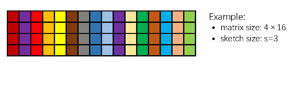
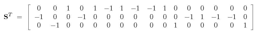
The matrix ${\bf S} \in \mathbb{R}^{n\times s}$ has exactly one nonzero entry in each row, and the entry can be either $+1$ or $-1$.In the above example, the sketching matrix ${\bf S}$ can be explicitly written as
3. In Memory Implementation
If the matrix ${\bf A}$ fits in memory, the above procedure can be straightforward implemented in a few lines of code. As we know, the loops in Python is slow, so this kind of implementation has the advantage of very few loops.
def countSketchInMemroy(matrixA, s):
    m, n = matrixA.shape
    matrixC = np.zeros([m, s])
    hashedIndices = np.random.choice(s, n, replace=True)
    randSigns = np.random.choice(2, n, replace=True) * 2 - 1 # a n-by-1{+1, -1} vector
    matrixA = matrixA * randSigns.reshape(1, n) # flip the signs of 50% columns of A
    for i in range(s):
        idx = (hashedIndices == i)
        matrixC[:, i] = np.sum(matrixA[:, idx], 1)
    return matrixC

s = 50 # sketch size, can be tuned
matrixC = countSketchInMemroy(matrixA, 50)
Let us test the quality of sketching. It is well known that the count sketch preserves the geometry of vectors. If the count sketch is implemented correctly, then for all $i = 1$ to $m$, $\|{\bf c}_{i:}\|$ should be close to $\|{\bf a}_{i:}\|$, and the closeness increase with $s$.
# Test
# compare the l2 norm of each row of A and C
rowNormsA = np.sqrt(np.sum(np.square(matrixA), 1))
print(rowNormsA)
rowNormsC = np.sqrt(np.sum(np.square(matrixC), 1))
print(rowNormsC)
4. Streaming Implementation
The matrix ${\bf A}$ is normally too large to fit in memory, but the sketch ${\bf C}$ can fit in memory. In such situation, we can read ${\bf A}$ in a streaming fashion, that is, keep only one column of ${\bf A}$ in memory at a time. The algorithm can be described as follows.
- Initialize ${\bf C}$ to be $m\times s$ all-zeros matrix;
- For $j = 1$ to $n$:
- read ${\bf a}_{:j}$ to memory;
- uniformly sample $h$ from $\{1, \cdots , s\}$;
- uniformly sample $g$ from $\{+1, -1\}$;
- add $g \cdot {\bf a}_{:j}$ to the $h$-th column of ${\bf C}$.
We implement the algorithm in the following. To make the code readable, we avoid the file I/O operations. If ${\bf A}$ does not fit in memory, one can simply replace the 7th line "a = matrixA[:, j]" by the file operation "readline()" followed by parsing.
def countSketchStreaming(matrixA, s):
    m, n = matrixA.shape
    matrixC = np.zeros([m, s])
    hashedIndices = np.random.choice(s, n, replace=True)
    randSigns = np.random.choice(2, n, replace=True) * 2 - 1
    for j in range(n):
        a = matrixA[:, j]
        h = hashedIndices[j]
        g = randSigns[j]
        matrixC[:, h] += g * a
    return matrixC

s = 50 # sketch size, can be tuned
matrixC = countSketchStreaming(matrixA, s)
# Test
# compare the l2 norm of each row of A and C
rowNormsA = np.sqrt(np.sum(np.square(matrixA), 1))
print(rowNormsA)
rowNormsC = np.sqrt(np.sum(np.square(matrixC), 1))
print(rowNormsC)
5. Map-Reduce Implementation
The map-reduce implementation is essentially the same to the in-memory implementation. As the name suggests, it suits the map-reduce programming.
- Mapper
- Take a column of ${\bf A}$ as input and flip its sign with probability $50\%$;
- Sample an integer from $\{1, \cdots , s\}$;
- Emit the key-value pair, where the key is the integer and the value is the input column with potentially flipped sign.
- Reducer
- Reduce the key-value pairs by key and perform summation over the values (the vectors).
Remark. The communication cost is merely $O(ms)$ rather than $O(mn)$ for the following reason. The "reduceByKey()" operation first sums the vectors with the same key locally on each worker. Therefore, before the communication, each worker holds at most $s$ vectors.
The following implements the count sketch in Spark and has been tested.
def countSketchMapReduce(filepath, s):
    # load data
    rawRDD = sc.textFile(filepath)
    # parse string data to vectors
    vectorRDD = rawRDD.map(lambda l: np.asfarray(l.split()))
    # map the vectors to key-value pairs
    pairRDD = vectorRDD.map(lambda vect: (np.random.randint(0, s), (np.random.randint(0, 2) * 2 - 1) * vect ))
    # reducer
    vectList = pairRDD.reduceByKey(lambda v1, v2: v1+v2).map(lambda pair: pair[1]).collect()
    return np.asarray(vectList).T

s = 50 # sketch size, can be tuned
filepath = './data/letters.txt'
matrixC = countSketchMapReduce(filepath, s)